Left Skewed Histogram Understanding the Relationship Between Mean and MedianWhen analyzing data, a histogram can provide a visual representation of its distribution. One common type of distribution is a left-skewed or negatively skewed distribution, where the data tail extends to the left. In this topic, we will explore what a left-skewed histogram looks like, how the mean and median are affected in this type of distribution, and the key differences between the two measures of central tendency.
What is a Left Skewed Histogram?
A histogram is a graphical representation of the frequency distribution of a set of continuous data. The data is divided into bins, and the height of each bar represents the number of observations within each bin.
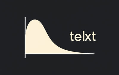
In a left-skewed histogram, the majority of the data points cluster on the right side of the graph, and the tail of the distribution extends toward the left. This skewness indicates that a few data points have relatively low values, pulling the distribution to the left. Left-skewed distributions are also referred to as negatively skewed because the left tail is longer than the right.
Characteristics of Left Skewed Data
To identify a left-skewed distribution in a histogram, look for the following characteristics
-
Most data points are concentrated on the right In a left-skewed histogram, the highest bars are on the right, and the frequency of data decreases as you move toward the left side of the graph.
-
A long tail on the left The left side of the histogram extends further than the right, indicating that a few data points have values much lower than the majority.
-
Asymmetry The distribution is not symmetrical. The bulk of the data is skewed towards the right side of the graph, while the left side has fewer data points that are more spread out.
Understanding Mean and Median in a Left Skewed Distribution
When analyzing data, the mean and median are two commonly used measures of central tendency, which describe the ‘center’ of a data set. However, in a left-skewed distribution, the mean and median behave differently, and it’s important to understand their relationship.
1. The Mean in a Left Skewed Distribution
The mean is calculated by summing all data points and dividing by the number of data points. In a left-skewed distribution, the mean is pulled in the direction of the tail, which is to the left. This means the mean will typically be less than the median in a left-skewed distribution.
Here’s why Since the tail contains extreme values that are lower than the majority of the data, these values drag the mean downward. The result is that the mean is often closer to the lower end of the scale than the median.
For example, imagine a set of incomes where most people earn between $30,000 and $50,000, but a few people earn significantly lower amounts, such as $10,000. These lower values would pull the mean down, even though most people earn higher amounts.
2. The Median in a Left Skewed Distribution
The median is the middle value when the data is arranged in numerical order. In a left-skewed distribution, the median is typically greater than the mean. This is because the median is less affected by extreme values (outliers) than the mean. In the case of a left-skewed distribution, the median is located in the center of the bulk of the data, which is on the right side of the graph.
Unlike the mean, the median represents the point where half of the data values lie below and half lie above. Since the extreme low values in the tail have little influence on the median, it remains higher than the mean.
Relationship Between Mean and Median in Left Skewed Distributions
In a left-skewed distribution, the general rule is that the mean is always less than the median. This happens because
-
The mean is sensitive to all data points, including the extreme low values in the left tail.
-
The median, being the middle value, is less affected by these extreme values and stays closer to the center of the data.
Thus, when you analyze a left-skewed histogram, you will notice that the mean is typically pulled to the left of the median.
Practical Example Left Skewed Data
Let’s consider a practical example to better understand the relationship between mean and median in a left-skewed distribution.
Imagine a data set that represents the ages of people at a retirement party. Most of the attendees are in their 60s and 70s, but a few younger guests are invited, such as their children, who are in their 20s. The ages of the older guests create a cluster toward the right of the histogram, while the younger guests create a long tail toward the left.
-
Mean Age The mean will be affected by the younger ages and will be lower than the median. For instance, if the average age of the guests is 60, the younger guests will pull the mean down.
-
Median Age The median, on the other hand, will be higher than the mean. Since the median represents the middle value of the data, it will be less influenced by the younger ages and will likely fall in the 60s or 70s, where most of the guests are.
How to Identify a Left Skewed Histogram
To visually identify a left-skewed histogram, look for these signs
-
The peak of the histogram is on the right, with most of the data clustering there.
-
The left tail of the histogram is longer, indicating that there are fewer but more extreme low values.
-
The distribution is asymmetric, with a noticeable drop-off on the right side and a gradual decline on the left.
A left-skewed histogram presents a distribution where the majority of the data values are concentrated on the right side, and the tail extends to the left. In such a distribution, the mean is typically less than the median due to the influence of extreme low values. Understanding this relationship helps in interpreting statistical data and making informed decisions based on the type of distribution you are dealing with.
When analyzing data in a left-skewed distribution, always consider both the mean and median to get a clearer picture of the data’s central tendency. By examining these two measures together, you can better understand the impact of extreme values on your data set and make more accurate conclusions.